1. Loss function(손실함수)
- Loss function은 classifier가 얼마나 잘 수행해내는지 알려줌
- weight 값을 판단하는 기준이 됨
- loss will be high, if we’re doing a poor job of classifying the training data
1) Multiclass Support Vector Machine loss (Hinge loss)
- (x_i, y_i)에서 x_i는 image, y_i는 (integer) label을 의미. 이때 scores vector: s=f(x_i, W)
- SVM loss는 다음과 같이 구한다

- s_j는 잘못된 label의 score, s_yi는 제대로 된 label의 score 의미. 1은 safety margin
- s_j – s_yi + 1 = s_j – (s_yi – 1). (correct label score – 1)보다 큰 incorrect label score가 있다면 loss는 0보다 크게 됨
- 가능한 loss의 min 값은 0, max 값은 무한대
- 만약 j=y_i인 경우도 포함한다면 loss값이 모두 1씩 증가하여 loss의 평균 값도 1 증가
- 전체 dataset에 대한 loss 값은 평균 낸 값

- 일반적으로 weight 값은 작은 값으로 초기화 -> score 값이 0에 가까운 값으로 나타남 -> 이때의 SVM loss는 max(0, 0-0+1) = 1이므로 초기의 전체 SVM loss 값은 (class – 1) -> sanity check에 이용됨
- squared hinge loss는 다음과 같다

- 제곱을 해서 non linear하게 되고, 차이가 생김
- 제곱을 하지 않은 hinge loss가 일반적이지만 경우에 따라 squared hinge loss를 사용하기도 함
- Multiclass SVM loss example code

Regularization
- unique한 weight 값을 지정해주기 위해 regularization 개념 등장

- Data loss : training dataset에 최적화하려고 함
- Regularization : test data에 최대한 일반화하려고 함
- -> data에 fit하고 가장 최적화된 weight값을 추출
- weight regularization을 더해주면 training data에 대한 정확도는 안 좋아지겠지만 test data에 대한 정확도는 좋아짐
L2 regularization
- weight 값을 0에 가깝도록 유도
- weight를 최대한 spread out 해서 모든 데이터 값의 input feature들을 고려함
- “diffuse over everything” 동일한 score라면 weight가 최대한 spread out된 것을 선호함
λ 값
- 높으면 모델이 단순해짐
- underfitting 위험 존재
- 낮으면 모델이 복잡해짐
- overfitting 위험 존재
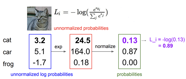
2) Softmax classifier
- scores = unnormalized log probabilities of the classes
- s = f(x_i;W)
- Softmax loss(Cross entropy loss)는 다음과 같이 구한다
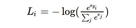
- L_i의 가능한 min값은 0, max는 무한
- weight값이 초기에 0에 가까운 값으로 초기화될 때 loss는 -log(1/class) -> sanity check에 이용
3) Softmax vs. SVM

- datapoint의 score 값을 약간 변경했을 때,
- softmax는 데이터에 민감해서 모든 data 값을 다 고려하기 때문에 loss 값이 변함
- svm은 데이터에 둔감해서 data 값들이 변하게 되더라도 loss 값은 변하지 않음
2. Optimization
- loss를 minimize하는 최적의 weight를 찾아가는 과정
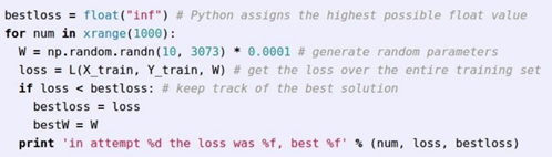
Strategy 1: Random search
- 절대로 사용해서는 안되는 전략 very bad idea
Strategy 2: Follow the slopenumerical gradient
numerical gradient
- evaluate the gradient numerically
- 1차원인 경우

- 다차원인 경우
- gradient는 vector로 나타남
- approximate, slow, easy to write
analytic gradient
- use calculus to compute gradient
- exact, fast, error-prone3. Gradient Descent

- step size는 learning rate이라고도 불림.
- Learning rate와 regularization strength는 모두 hyperparameter이라 최적의 값을 찾는 게 매우 중요함

- 임의의 위치에서 가운데 빨간색 지점으로 가는 것, 즉 기울기가 0에 가까운 지점으로 가는 것이 목표
- full batch gradient descent: training set 전체를 이용
- mini batch gradient descent: small portion of the training set 이용
Stochastic Gradient Descent (SGD)
- mini batch gradient descent의 대표적인 예
- approximate sum using a minibatch of examples 32/64/128 common
4. Image features - CNN 등장 이전의 방식들
- CNN이 나오기 전 image classification 이 이루어진 방식
- image feature를 추출한 다음에 concatenation 시켜서 하나의 giant column vector를 만들어 linear classifier 적용
example: color histogram
- 모든 pixel들의 color를 추출
example: histogram of oriented gradients (HoG)
- edge들의 orientation feature를 추출
- 방향값을 히스토그램으로 표현
example: bag or words
- 이미지의 random patch 잘라 냄 -> 이미지에서 각도, 색깔 등의 image feature 추출 -> 새로운 이미지가 들어오면 이미지를 잘라내어 cluster과 비교
이처럼 특징을 추출해서 linear classifier에 적용하는 방식이 아니라, model이 스스로 이미지 특징을 뽑아내도록 하는 것이 CNN
'Deep Learning > CS231n' 카테고리의 다른 글
| CS231n 6강 summary (0) | 2021.06.23 |
|---|---|
| CS231n 5강 summary (0) | 2021.06.23 |
| CS231n 2강 summary (0) | 2021.06.23 |
| CS231n 1강 summary (0) | 2021.06.23 |
| cs231n 4주차 예습과제 (0) | 2021.05.02 |